class: center, middle, inverse, title-slide # STA130H1F ## Class #7 ### Prof. Nathan Taback ### 2018-10-21 --- --- ## Purpose of today's class - Review some material and ideas for the test. - Not 100% comprehensive. - What else should you study? - All lecture slides, weekly practice problems. --- ## Structure of test The test is a combination of: * multiple choice * fill in the blanks * short answer (explain why / apply) * answers that require you to write some sentences --- # Lightning Round --- ## Lightning Round Question 1 <font size="4"> A clinical oncologist is investigating the efficacy of a new treatment on reduction in tumour size. She randomly assigns patients to the new treatment or old treatment and compares the mean of the reduction in tumour size between the two groups. She carries out a statistical test and the P-value is 0.001. How many of the following are valid interpretations of the P-value? <br> <br> I. The probability of observing a difference between the treatment groups as large or larger than she observed if the new treatment has the same efficacy as the old treatment. <br> II. The probability that the new treatment works the same as the old treatment. <br> III. The probability that the new treatment, on average, reduces tumour size more than the old treatment. <br> <br> A. None <br> B. One <br> C. Two <br> D. Three <br> </font> --- ## Lightning Round Question 2 Fill in the respective blanks: Suppose we wish to test the null hypothesis that a Yoga method does not have an effect on blood pressure versus the alternative that it does have an effect. A <font color="blue" .underline[XX]</font> error would be made by concluding that the Yoga method <font color="blue" .underline[XX]</font> on blood pressure if in fact the Yoga method <font color="blue" .underline[XX]</font> on blood pressure. A. Type 2; does have an effect; does have an effect B. Type 2; does not have an effect; does not have an effect C. Type 1; does have an effect; does not have an effect D. Type 1; does not have an effect; does not have an effect E. P-value error; does have an effect; does not have an effect --- ## Lightning Round Question 3 In statistical inference, we want to make conclusions about what we think about the **theoretical world** or **population** based on what we've observed in the **real world** (data, typically observed on a random sample). Do the following items exist in the theoretical world or the real world? * Observed value of test statistic * Parameter * Null hypothesis (and alternative hypothesis) * Simulated values of the test statistic under the null hypothesis * P-value --- ## Lightning Round Question 4 Consider the following R code. ```r Tosses <- c("H","H","T", "H") myfunction <- function(x){ result <- sample(x = x, replace = FALSE) sum(result == "T") } myfunction(Tosses) ``` Which of the following is the value that `myfunction(Tosses)` will return: (I) 0 (II) 1 (III) 2 (III) 3 (IV) 4 --- # Case Study: American Community Survey 2012 --- ## Case Study: American Community Survey 2012 The American Community Survey is conducted by the US Census Bureau each year on a random sample of 3.5 million households. Findings from the survey influence the allocation of more than $400 billion in federal and state funds. The dataset `acs12` is a random sample from the people who completed the American Community Survey in 2012. --- Here is a look at the data and some of the variables we will consider later: ```r glimpse(acs12) ``` ``` ## Observations: 2,000 ## Variables: 13 ## $ income <int> 60000, 0, NA, 0, 0, 1700, NA, NA, NA, 45000, NA, ... ## $ employment <fct> not in labor force, not in labor force, NA, not i... ## $ hrs_work <int> 40, NA, NA, NA, NA, 40, NA, NA, NA, 84, NA, 23, N... ## $ race <fct> white, white, white, white, white, other, white, ... ## $ age <int> 68, 88, 12, 17, 77, 35, 11, 7, 6, 27, 8, 69, 69, ... ## $ gender <fct> female, male, female, male, female, female, male,... ## $ citizen <fct> yes, yes, yes, yes, yes, yes, yes, yes, yes, yes,... ## $ time_to_work <int> NA, NA, NA, NA, NA, 15, NA, NA, NA, 40, NA, 5, NA... ## $ lang <fct> english, english, english, other, other, other, e... ## $ married <fct> no, no, no, no, no, yes, no, no, no, yes, no, no,... ## $ edu <fct> college, hs or lower, hs or lower, hs or lower, h... ## $ disability <fct> no, yes, no, no, yes, yes, no, yes, no, no, no, n... ## $ birth_qrtr <fct> jul thru sep, jan thru mar, oct thru dec, oct thr... ``` --- ```r table(acs12$employment) ``` ``` ## ## not in labor force unemployed employed ## 656 106 843 ``` ```r table(acs12$edu) ``` ``` ## ## hs or lower college grad ## 1439 359 144 ``` --- ### Case study question 1 Describe the data frames that are created by each of the following commands: ```r labor_force <- acs12 %>% filter(!is.na(employment)) %>% filter(employment == "employed" | employment == "unemployed") employed <- labor_force %>% filter(employment == "employed") employed <- employed %>% mutate(edu2 = recode(edu, "hs or lower" = "hs_or_lower", "college" = "more_than_hs", "grad" = "more_than_hs")) cat_vars <- acs12 %>% select(employment, race, gender, citizen, lang, married, edu, disability, birth_qrtr) ``` --- ### Case study question 2 We've used these plot geometries: `geom_bar, geom_boxplot, geom_dotplot, geom_histogram, geom_line, geom_point, geom_vline` Recall this plot vocabulary: * Bar plots: modes, frequency * Histograms / boxplots: centre, spread, modes (unimodal, bimodal, multimodal, no mode), frequency, symmetric / left-skewed / right-skewed, outliers * Scatterplots: strong / weak / no relationship, linear (positive or negative) / nonlinear relationship, and outliers. --- On the next several slides are a number of plots, each constructed from the dataset `employed`. For each: * What type of plot is it? * What `ggplot` geometry is used? * What is the purpose of the plot? * Describe the distribution(s) of the variable(s). --- ## Plot 1 <!-- --> * What type of plot is it? * What `ggplot` geometry is used? * What is the purpose of the plot? * Describe the distribution(s) of the variable(s). --- ## Plot 2 <!-- --> * What type of plot is it? * What `ggplot` geometry is used? * What is the purpose of the plot? * Describe the distribution(s) of the variable(s). --- ## Plot 3 <!-- --> * What type of plot is it? * What `ggplot` geometry is used? * What is the purpose of the plot? * Describe the distribution(s) of the variable(s). * What is the difference in these histograms? --- ### Case study question 3 We have looked at simulations to estimate P-values in hypothesis tests. -- The hypothesis tests we have considered are: - single proportion - comparing two proportions - comparing two statistics for continuous variables (e.g., means, medians, sd) -- The purpose of the simulation was to examine possible values of a statistic under an assumption. Two cases of this were considered: -- - simulate outcomes for a proportion - simulate the difference in a statistic between groups --- ### Case study question 3 Below is code for three simulations. For each: * What is the purpose of the simulation? * State the hypothesis test being conducted? * What are the null and alternative hypotheses? * Estimate the P-value from the values plotted. * What is your conclusion? --- ### Some statistics that might be useful ```r labor_force %>% group_by(employment) %>% summarise(n_group = n()) %>% mutate(percent = n_group / sum(n_group)) ``` ``` ## # A tibble: 2 x 3 ## employment n_group percent ## <fct> <int> <dbl> ## 1 unemployed 106 0.112 ## 2 employed 843 0.888 ``` --- ```r employed %>% group_by(edu2) %>% summarise(median(income)) ``` ``` ## # A tibble: 2 x 2 ## edu2 `median(income)` ## <fct> <dbl> ## 1 hs_or_lower 23000 ## 2 more_than_hs 46000 ``` ```r employed %>% group_by(edu2) %>% summarise(mean(income)) ``` ``` ## # A tibble: 2 x 2 ## edu2 `mean(income)` ## <fct> <dbl> ## 1 hs_or_lower 29963. ## 2 more_than_hs 65010. ``` --- ### Simulation 1 ```r repetitions <- 100 x <- rep(NA, repetitions) n <- as.numeric(labor_force %>% summarize(n())) for (i in 1:repetitions) { sim <- sample(c("unemployed", "employed"), size = n, prob = c(0.089, 1 - 0.089), replace = TRUE) sim_stat <- sum(sim == "unemployed") / n x[i] <- as.numeric(sim_stat) } ``` * What is the purpose of the simulation? * State the hypothesis test being conducted? What is `\(H_0, H_A\)`? * What are the null and alternative hypotheses? --- <!-- --> - What does the y-axis represent? - Estimate the P-value. - What do you conclude? --- ### Simulation 2 ```r set.seed(1) repetitions <- 100 x <- rep(NA, repetitions) for (i in 1:repetitions) { sim <- employed %>% mutate(edu2 = sample(edu2)) sim_stat <- sim %>% group_by(edu2) %>% summarise(medians = median(income)) %>% summarise(diff(medians)) x[i] <- as.numeric(sim_stat) } ``` * What is the purpose of the simulation? * State the hypothesis test being conducted? What is `\(H_0, H_A\)`? * What are the null and alternative hypotheses? --- 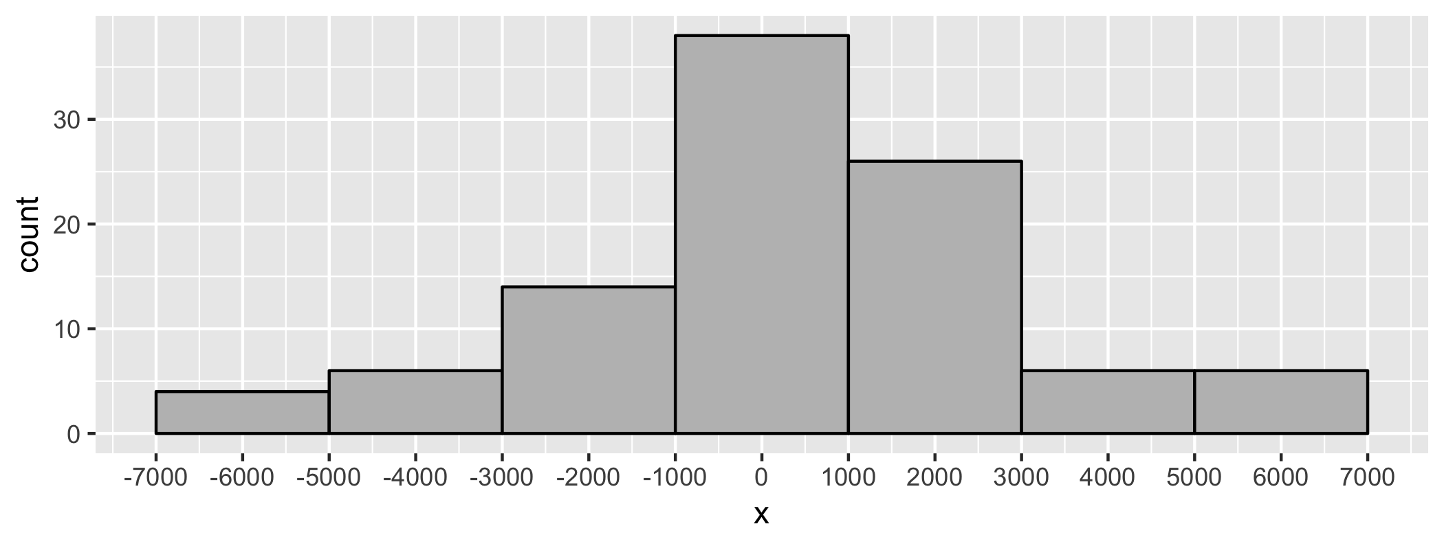<!-- --> - Estimate the P-value. - What do you conclude? --- ### Simulation 3 ```r set.seed(1) repetitions <- 100 x <- rep(NA, repetitions) for (i in 1:repetitions) { sim <- employed %>% mutate(edu2 = sample(edu2)) sim_stat <- sim %>% group_by(edu2) %>% summarise(mean = mean(income)) %>% summarise(diff(mean)) x[i] <- as.numeric(sim_stat) } ``` * What is the purpose of the simulation? * State the hypothesis test being conducted? What is `\(H_0, H_A\)`? * What are the null and alternative hypotheses? --- 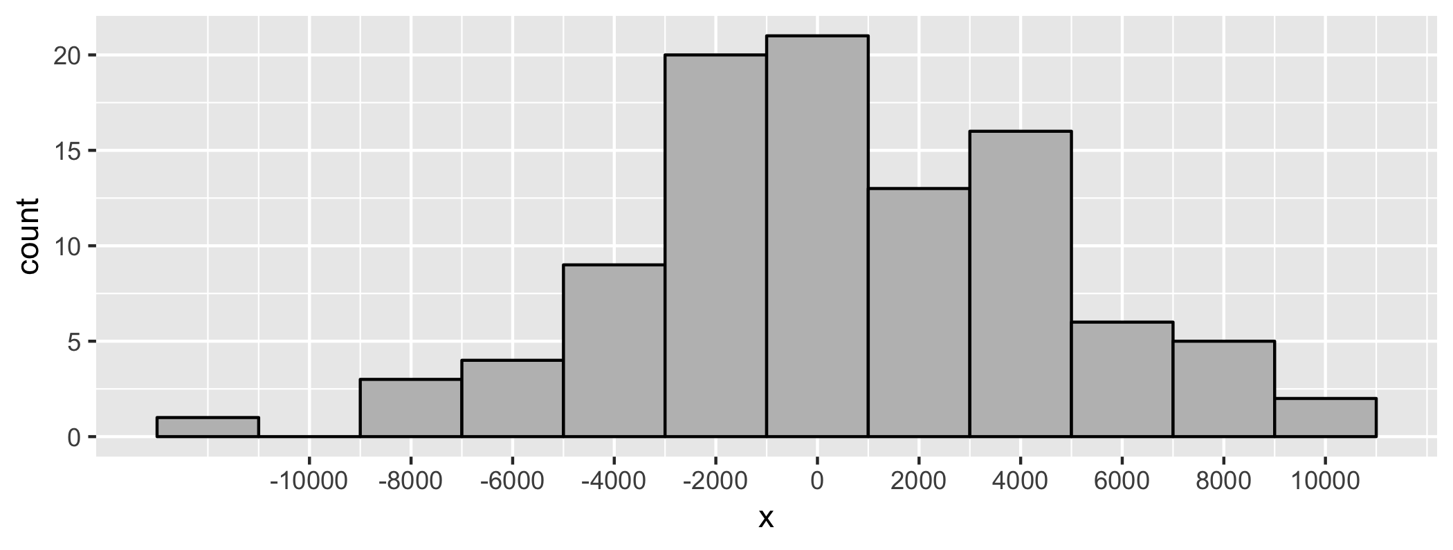<!-- --> - Estimate the P-value. - What do you conclude?