class: center, middle, inverse, title-slide # STA130H1F ## Class #9 ### Prof. Nathan Taback ### 2018-11-12 --- ## Today's Class - Supervised versus Unsupervised Learning - Classification Trees - Interpreting a Classification Tree - Geometric Interpretation of a Classification Trees - Classification Tree Methodology - Training and Testing Classification Trees - Accuracy of Classification Trees - ROC Curves --- # Learning from Data --- ## Supervised versus Unsupervised Learning - Many statistical learning problems fall into one of two categories: supervised or unsupervised. - In supervised learning problems there is a response measurement `\(y\)` that we would like to __predict__, based on variables `\(x_1, x_2, \ldots, x_p\)`. - Variables are often called features, predictors, covariates, independent variables, or inputs. - Response measurements are often called outputs, labels, or dependent variables. --- ## Image Classification Example .pull-left[ - Imagine that we want to build a system that can classify images as containing, say, a house, a car, a person or a pet. - We first collect a large data set of images of houses, cars, people and pets, each labelled with its category. - Convert the images to input variables. ] .pull-right[  ```r library(jpeg) # get RGB intensity 0 - 255 img <- readJPEG("pika.jpg") img[40:41,51:52,1] ``` ``` ## [,1] [,2] ## [1,] 0.1568627 0.015686275 ## [2,] 0.2745098 0.003921569 ``` ] --- ## Image Classification Example - "Train" an algorithm. - The algorithm produces an output in the form of a vector of scores, one for each category. - We want the desired category to have the highest score of all categories, but this is unlikely to happen before training. - We next compute the error between the output scores and the true scores. --- # Classification Trees --- ## Classification Trees - Data was collected on 50 cancer patients to investigate the effectivness (Yes/No) of a treatment. - Two quantitative variables, `\(x_i \in (0,1), i=1,2\)`, are considered to be important predictors of effectiveness. --- ## Classification Trees ```r library(rpart) library(partykit) tree <- rpart(type_cat ~ x1 + x2, data = dat) plot(as.party(tree), type = "simple", gp = gpar(cex = 0.8)) ``` <!-- --> --- ## Interpreting a Classification Tree .pull-left[ <!-- --> - This classification tree has five nodes, and three of these nodes are __terminal nodes__. - Terminal nodes are indicated by rectangular boxes, and nonterminal nodes are indicated by ovals. ] .pull-right[ - If a subject has `\(x1 < 0.211\)` then the prediction is that effectiveness = Yes (i.e., the treatment is effective). 7 subjects have `\(x1 < 0.211\)` and 42.9% (3 subjects) have effectiveness = No, and 57.1% (4 subjects) have effectiveness = Yes. - If a subject has `\(x1 \geq 0.211\)` and `\(x2 < 0.586\)` then the prediction is that effectiveness = No. 16 subjects have `\(x1 \geq 0.211\)` and `\(x2 < 0.586\)` and 18.8% (3 subjects) have effectiveness = Yes, and 81.2% (13 subjects) have effectiveness = No. ] --- ## Geometric Interpretation of a Classification Trees A scatter plot of `\(x1, x2\)` is shown below where each point is labelled by effectivness. ```r ggplot(dat, aes(x1, x2, shape = factor(type_cat), colour = factor(type_cat))) + geom_point(size = 2) + theme_minimal() + scale_color_discrete(name = "Effectiveness", breaks = c("Yes", "No")) + scale_shape_discrete(name = "Effectiveness", breaks = c("Yes", "No")) ``` <!-- --> --- ## Geometric Interpretation of a Classification Tree .pull-left[ - An equivalent way of looking at this tree is that it divides the unit square into rectangles. - The division is recursive since it first __splits__ the rectangle into two pieces, then it may __split__ each of these rectangles into two pieces, etc. ] .pull-right[ <!-- --> <!-- --> ] --- ## Classification Tree Methodology 1. A set of binary questions. For example, is `\(\{x1 < 0.5\}\)`? 2. A method to evaluate if a split is "good". 3. A rule to stop-splitting. 4. A rule for assigning every terminal node to a category (i.e., Yes or No). --- ## Classification Tree Methodology - The standard set of questions - Suppose that we have `\(M\)` variables `\(x_1,x_2,\dots,x_M\)` which can be a mixture of of continuous and categorical variables. - Each split depends on the value of only a single variable. - For each continuous variable `\(x_m\)`, a split is of the form: is `\(\{x_m \le c \}?\)` or is `\(\{x_m > c \}?,\mbox{ } c \in (-\infty,\infty).\)` - If `\(x_m\)` is categorical, taking values, say, in `\(\{b_1, b_2, \ldots, b_L\}\)` then splits are of the form: is `\(\{x_m \in S\}?\)` as `\(S\)` ranges over all subsets of `\(\{b_1, b_2, \ldots, b_L\}\)`. --- ## Classification Tree Methodology - The standard set of questions - At each node the tree algorithm searches through the variables one by one. - For each variable it finds the 'best' split. - Then the algorithm compares the `\(M\)` best single variable splits and selects the best of the best. --- ## Classification Tree Methodology - The Splitting and Stop Splitting Rule In order to perform recursive binary splitting: - A node of a tree is said to be _impure_ when all classes are equally mixed together. - For example, a node that had 50% of subjects with effectiveness = No and 50% of subjects with effectiveness = Yes. - Two popular measures of impurity, `\(i(t)\)`, for node `\(t\)` are Gini, and Entropy: $$ Gini(t) = 1- \{(w_1(t))^2+(w_2(t))^2\}, \mbox{ } \\ Entropy(t) = -\{w_1(t)\log_2(w_1(t)) + w_2(t)\log_2(w_2(t))\},$$ where `\(w_i(t)\)` is the fraction of records belonging to class `\(i\)` at node `\(t\)`. --- ## Classification Tree Methodology - The Splitting and Stop Splitting Rule - The "goodness" of a split is the decrease in impurity `\(\Delta I\)`. The maximum decrease in impurity is defined as the best split. - A simple stop-splitting rule is to set a threshold, say `\(\beta >0\)`, and declare a node terminal if `\(\Delta I < \beta.\)` --- ## Example: Predicting High Earners - What factors can be used to predict if a person is a high earner? - Capital gains tax is the tax paid on profit from the sale of an asset (e.g., stock, bond, property). - Does the amount of capital gains tax predict if a person is a higher earner? --- ## Example: Predicting High Earners ```r census %>% ggplot(aes(income)) + geom_bar(colour = "black", fill = "grey", alpha = 0.5) + theme_minimal() ``` <!-- --> --- ## Example: Predicting High Earners ```r census %>% ggplot(aes(capital.gain)) + geom_histogram(colour = "black", fill = "grey", alpha = 0.5) + theme_minimal() ``` <!-- --> --- ## Example: Predicting High Earners ```r census %>% ggplot(aes(x = capital.gain, y = income)) + geom_count(position = position_jitter(width = 0, height = 0.1), alpha = 0.5) + scale_x_log10(labels = scales::dollar, breaks = c(0,1000,5000,100000)) + theme_minimal() + theme(legend.position = "none") ``` <!-- --> --- ## Example: Predicting High Earners Classify people with capital gains less than $5000 as low earners and greater than $5000 as high earners. 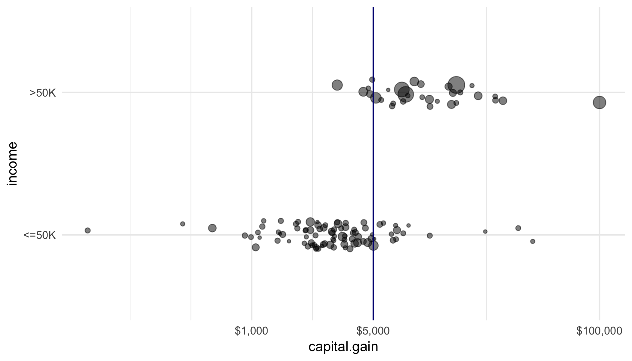<!-- --> --- # Evaluating Classification Tree Models --- ## Resampling Methods in Statistics - There are several types of resampling methods in statistics. - The randomization and permutation tests have been used to calculate p-values. - The bootstrap has been used to calculate confidence intervals. - Resampling can also be used to assess the accuracy of a prediction model. --- ## Validation Set Approach - Suppose that we would like to estimate the test error associated with fitting a particular statistical learning method on a set of observations. - The validation set approach involves randomly dividing the available set of observations into two parts: a training set and a validation set or hold-out set. - The tree model is fit on the training set, and the fitted model is used to predict the responses for the observations in the validation set. --- ## Validation Set Approach The validation set approach has two drawbacks: 1. The test error rate can be variable since it depends on which observations are included in the training and validation set. 2. Only a subset of the observations are used to fit the tree. Statistical methods perform worse when trained on fewer observations. Thus, the validation set approach may tend to overestimate the test error rate. --- ## Training and Testing Classification Trees - Separate the data set into two data sets by randomly selecting rows. - A sample of 80% of the rows will become the _training_ data set. - The remaining 20% will be set aside as the _testing_ (or "hold-out") data set. - There are no formal rules about the percentage of data that should be training and testing. --- ## Training and Testing Classification Trees ```r set.seed(364) # number of observations in census data n <- nrow(census) n ``` ``` ## [1] 32561 ``` ```r # random sample of 20% of row indexes test_idx <- sample.int(n, size = round(0.2 * n)) # training data is all observations except from training row indexes train <- census[-test_idx, ] nrow(train) ``` ``` ## [1] 26049 ``` ```r # test data test <- census[test_idx, ] nrow(test) ``` ``` ## [1] 6512 ``` --- ## Training and Testing Classification Trees ```r train <- train %>% mutate(income = factor(income), workclass = factor(workclass), education = factor(education), marital.status = factor(marital.status), occupation = factor(occupation), relationship = factor(relationship), race = factor(race), sex = factor(sex)) test <- test %>% mutate(income = factor(income), workclass = factor(workclass), education = factor(education), marital.status = factor(marital.status), occupation = factor(occupation), relationship = factor(relationship), race = factor(race), sex = factor(sex)) ``` --- ## Example: Predicting High Earners ```r train %>% group_by(income) %>% summarise(n = n()) %>% mutate(relfreq = round(n/sum(n),2)) ``` ``` ## # A tibble: 2 x 3 ## income n relfreq ## <fct> <int> <dbl> ## 1 <=50K 19732 0.76 ## 2 >50K 6317 0.24 ``` - If we predict that everyone in the training data earns less than 50K then we will be correct with 76% accuracy. --- ## Example: Predicting High Earners - If we use the plot of income versus capital gains and we use the split $5000 capital gains then the accuracy of our prediction changes to: ```r split <- 5000 confusion_dat <- train %>% mutate(hi_cap_gains = capital.gain >= split) %>% group_by(income, hi_cap_gains) %>% summarise(n = n()) confusion_dat ``` ``` ## # A tibble: 4 x 3 ## # Groups: income [?] ## income hi_cap_gains n ## <fct> <lgl> <int> ## 1 <=50K FALSE 19613 ## 2 <=50K TRUE 119 ## 3 >50K FALSE 5115 ## 4 >50K TRUE 1202 ``` --- ## Example: Predicting High Earners - Confusion Matrix - The data can be displayed as a confusion matrix. ```r confusion <- matrix(confusion_dat$n,byrow = F, ncol = 2) rownames(confusion) <- c("Cap Gains < $5000", "Cap Gains >= $5000") colnames(confusion) <- c("Income <50K", "Income >= 50K") confusion ``` ``` ## Income <50K Income >= 50K ## Cap Gains < $5000 19613 5115 ## Cap Gains >= $5000 119 1202 ``` - The overall accuracy has increased to (19613+1202)/(19613+1202+119+5115) = 0.799071. --- ## Example: Predicting High Earners - Confusion Matrix - Is $5000 the "best" split of capital gains to predict income? - We want to find the value of capital gains such that it "splits" the data into low/high income. - There are several measures that are used to find measure the goodness of a split. - Two popular measures are the Gini index and Entropy. --- ## Example: Predicting High Earners - Plotting ```r library(rpart) tree <- rpart(income ~ capital.gain, data = train, parms = list(split = "gini")) tree ``` ``` ## n= 26049 ## ## node), split, n, loss, yval, (yprob) ## * denotes terminal node ## ## 1) root 26049 6317 <=50K (0.75749549 0.24250451) ## 2) capital.gain< 5095.5 24784 5115 <=50K (0.79361685 0.20638315) * ## 3) capital.gain>=5095.5 1265 63 >50K (0.04980237 0.95019763) * ``` ```r library(partykit) plot(as.party(tree),type = "simple", gp = gpar(cex = 0.5)) ``` 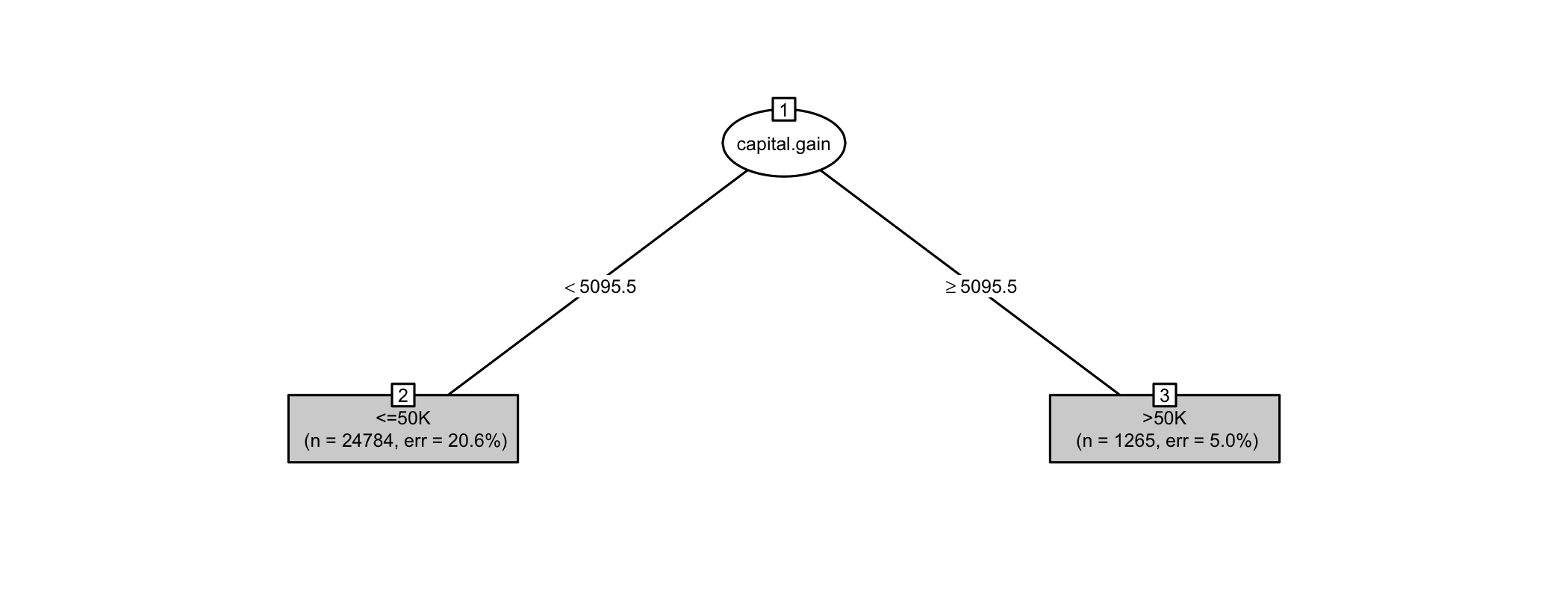<!-- --> --- ## Classification Tree Accuracy - The test data was not used to build the tree. - If the tree only works well on the data that was used to build the tree, and poorly on a new set of data then the model (i.e., tree) is said to be __overfit__. - This is the rationale behind using part of the data to buid the model (i.e., tree) and using another part to test the accuracy of the tree. --- ## Classification Tree Accuracy - The accuracy of the classification tree model is captured in a table of actual (observed) incomes versus the predicted incomes for each person. - The table is often called a __confusion matrix__. ```r predicted_tree <- predict(object = tree, newdata = test, type = "class") table(predicted_tree,test$income) # confusion matrix ``` ``` ## ## predicted_tree <=50K >50K ## <=50K 4969 1230 ## >50K 19 294 ``` - The overall accuracy of the tree is (4969 + 294)/(4969 + 1230 + 19 +294) = 0.8082002. - For those that earned <=50K the accuracy is: 4969/(4969 + 19) = 0.9961909. - For those that earned >50K the accuracy is: 294/(294 + 1230) = 0.1929134. --- ## Classification Tree Accuracy Consider the confusion matrix: | Predicted | <= 50K | >50K | Total | |-----------|--------|------|-------| | <=50K | a | b | a+b | | >50K | c | d | c+d | | Total | a+c | b+d | N | N = (a + b + c + d). Assume we are trying to predict >50K. So this outcome will be considered positive, and <=50K is negative. - True positive rate (sensitivity): d/(b+d) - True negative rate (specificity): a/(a+c) - False positive rate: c/(a+c) - False negative rate: b/(b+d) - Accuracy: (a+d)/N --- ## Classification Tree Accuracy ```r predicted_tree <- predict(object = tree, newdata = train, type = "class") table(predicted_tree, train$income) # confusion matrix ``` ``` ## ## predicted_tree <=50K >50K ## <=50K 19669 5115 ## >50K 63 1202 ``` - Is there evidence of overfitting? --- ## Classification Trees - Picking the threshold value - It tried all possible values `\(c\)`, such that `capital gain` `\(\le c\)`. - $5095 was the one the value that gave the "best" separation between >50K and <=50K. --- ## Classification Trees - Adding more variables We have used only one variable to predict income, but we can use the other variables in the data to try and improve the accuracy. --- ## Classification Trees - Adding more variables ```r form <- as.formula("income ~ age + workclass + education + marital.status + occupation + relationship + race + sex + capital.gain + capital.loss + hours.per.week") mod_tree <- rpart(form, data = train) mod_tree ``` ``` ## n= 26049 ## ## node), split, n, loss, yval, (yprob) ## * denotes terminal node ## ## 1) root 26049 6317 <=50K (0.75749549 0.24250451) ## 2) relationship=Not-in-family,Other-relative,Own-child,Unmarried 14196 947 <=50K (0.93329107 0.06670893) ## 4) capital.gain< 7073.5 13946 706 <=50K (0.94937617 0.05062383) * ## 5) capital.gain>=7073.5 250 9 >50K (0.03600000 0.96400000) * ## 3) relationship=Husband,Wife 11853 5370 <=50K (0.54695014 0.45304986) ## 6) education=10th,11th,12th,1st-4th,5th-6th,7th-8th,9th,Assoc-acdm,Assoc-voc,HS-grad,Preschool,Some-college 8280 2769 <=50K (0.66557971 0.33442029) ## 12) capital.gain< 5095.5 7857 2355 <=50K (0.70026728 0.29973272) * ## 13) capital.gain>=5095.5 423 9 >50K (0.02127660 0.97872340) * ## 7) education=Bachelors,Doctorate,Masters,Prof-school 3573 972 >50K (0.27204030 0.72795970) * ``` --- ## Classification Trees - Adding more variables ```r library(partykit) plot(as.party(mod_tree),type = "simple", gp = gpar(cex = 0.4)) ``` <!-- --> ```r mod_tree ``` ``` n= 26049 node), split, n, loss, yval, (yprob) * denotes terminal node 1) root 26049 6317 <=50K (0.75749549 0.24250451) 2) relationship=Not-in-family,Other-relative,Own-child,Unmarried 14196 947 <=50K (0.93329107 0.06670893) 4) capital.gain< 7073.5 13946 706 <=50K (0.94937617 0.05062383) * 5) capital.gain>=7073.5 250 9 >50K (0.03600000 0.96400000) * 3) relationship=Husband,Wife 11853 5370 <=50K (0.54695014 0.45304986) 6) education=10th,11th,12th,1st-4th,5th-6th,7th-8th,9th,Assoc-acdm,Assoc-voc,HS-grad,Preschool,Some-college 8280 2769 <=50K (0.66557971 0.33442029) 12) capital.gain< 5095.5 7857 2355 <=50K (0.70026728 0.29973272) * 13) capital.gain>=5095.5 423 9 >50K (0.02127660 0.97872340) * 7) education=Bachelors,Doctorate,Masters,Prof-school 3573 972 >50K (0.27204030 0.72795970) * ``` --- ## Accuracy of Classification Tree ```r predicted_mod <- predict(mod_tree, newdata = test, type = "class") table(predicted_mod, test$income) ``` ``` ## ## predicted_mod <=50K >50K ## <=50K 4731 755 ## >50K 257 769 ``` - The overall accuracy is ... --- ## Accuracy of Classification Tree - Instead of predicting class we can predict probability. ```r predicted_tree <- predict(object = mod_tree, newdata = test, type = "prob") head(predicted_tree) ``` ``` ## <=50K >50K ## 1 0.7002673 0.2997327 ## 2 0.2720403 0.7279597 ## 3 0.7002673 0.2997327 ## 4 0.7002673 0.2997327 ## 5 0.7002673 0.2997327 ## 6 0.0212766 0.9787234 ``` ```r # if predicted prob of >50K is >=0.5 then predicted class is >50K # otherwise predicted class is <=50K m <- table(predicted_tree[,2] >= 0.5,test$income) row.names(m) <- c("Pred <50K","Pred >=50K") m ``` ``` ## ## <=50K >50K ## Pred <50K 4731 755 ## Pred >=50K 257 769 ``` --- ## Classification Tree Accuracy Since 24% of the sample earns >50K perhaps this is a more sensible cutoff for prediction. ```r predicted_tree <- predict(object = mod_tree, newdata = test, type = "prob") m <- table(predicted_tree[,2] >= 0.24,test$income) row.names(m) <- c("Pred <50K","Pred >=50K") m ``` ``` ## ## <=50K >50K ## Pred <50K 3370 166 ## Pred >=50K 1618 1358 ``` --- ## ROC Curves The ROC curve is a plot of the true positive rate versus the false positive rate for various cut-points. ```r pred <- ROCR::prediction(predictions = predicted_tree[,2], test$income) perf <- ROCR::performance(pred, 'tpr', 'fpr') perf_df <- data.frame(perf@x.values, perf@y.values) names(perf_df) <- c("fpr", "tpr") roc <- ggplot(data = perf_df, aes(x = fpr, y = tpr)) + geom_line(color = "blue") + geom_abline(intercept = 0, slope = 1, lty = 3) + ylab(perf@y.name) + xlab(perf@x.name) roc ``` 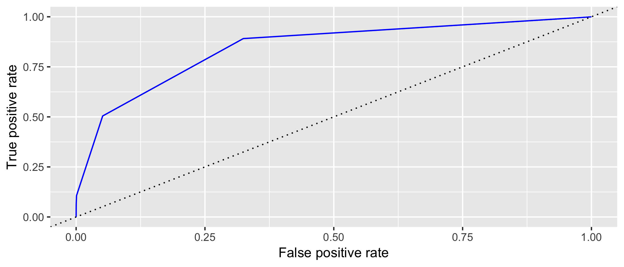<!-- --> --- ## ROC Curves .pull-left[ - The ROC curve is a plot of all possible threshold values for classification. - The upper-left corner represents a perfect classifier, which would have a true positive rate of 1 and a false positive rate of 0. - A random classifier would lie along the diagonal, since it would be equally likely to make either kind of mistake. ] .pull-right[ 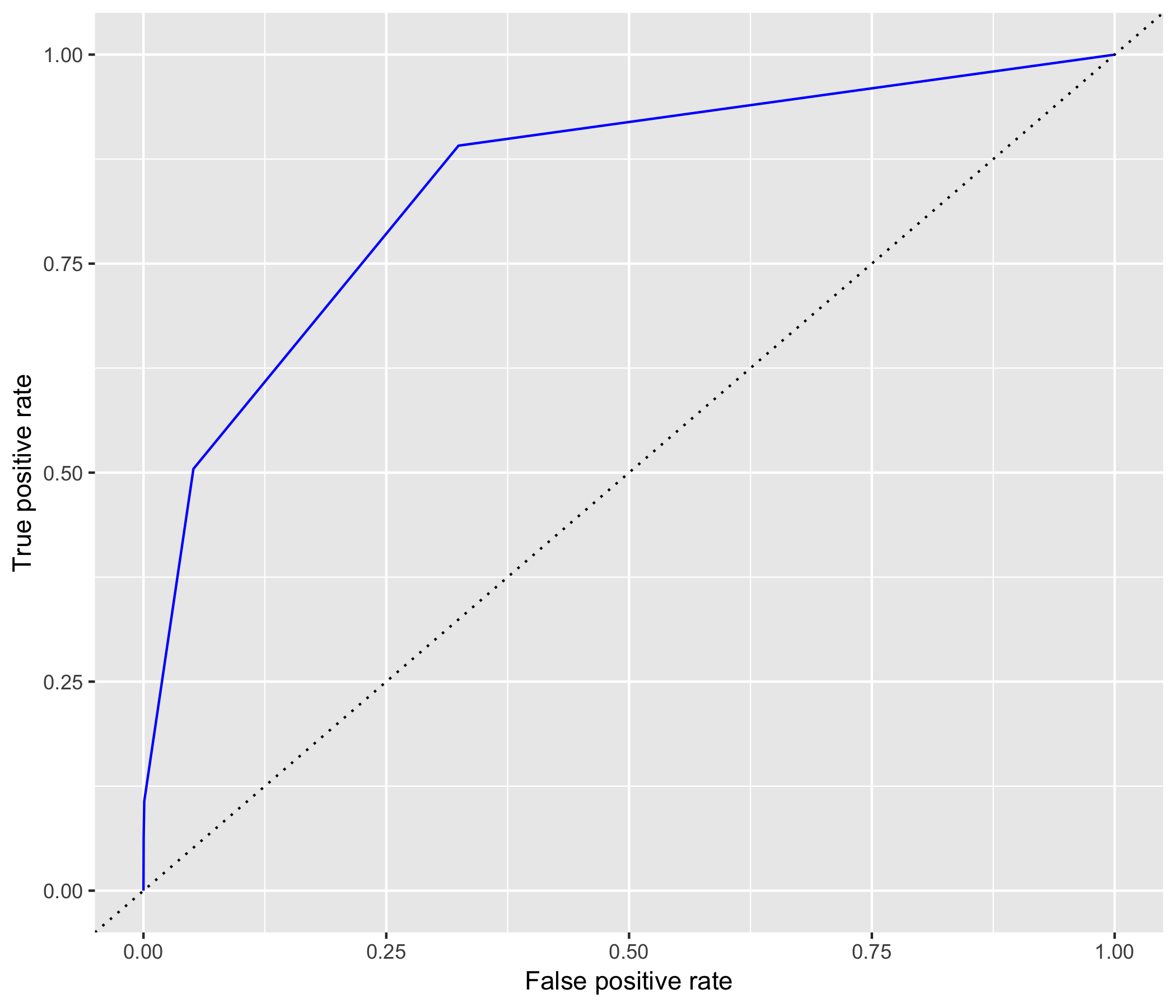<!-- --> ] --- ## ROC Curves The true positive rate and false positive rate for a tree classifier with cutpoint 0.5. ```r predicted_tree <- predict(object = mod_tree, newdata = test, type = "prob") m <- table(predicted_tree[,2] >= 0.50,test$income) row.names(m) <- c("Pred <50K","Pred >=50K") tpr_50 <- m[4]/sum(m[,2]) fpr_50 <- m[2]/sum(m[,1]) tpr_50 ``` ``` ## [1] 0.5045932 ``` ```r fpr_50 ``` ``` ## [1] 0.05152366 ``` --- ## ROC Curves The true positive rate and false positive rate for a tree classifier with cutpoint 0.24. ```r predicted_tree <- predict(object = mod_tree, newdata = test, type = "prob") m <- table(predicted_tree[,2] >= 0.24,test$income) row.names(m) <- c("Pred <50K","Pred >=50K") tpr_24 <- m[4]/sum(m[,2]) fpr_24 <- m[2]/sum(m[,1]) tpr_24 ``` ``` ## [1] 0.8910761 ``` ```r fpr_24 ``` ``` ## [1] 0.3243785 ``` --- ## ROC Curves The tree with a cutpoint of 0.5 is shown as the black dot and the tree with a cutpoint of 0.24 is shown as the red dot. ```r roc + geom_point(x = fpr_50, y = tpr_50, size = 3, colour = "black") + geom_point(x = fpr_24, y = tpr_24, size = 3, colour = "red") ``` <!-- -->